Received: Fri 11, Aug 2023
Accepted: Tue 17, Oct 2023
Abstract
Objective: To compare the performance of popular machine learning algorithms (ML) in mapping the sensorimotor cortex (SM) and identifying the anterior lip of the central sulcus (CS). Methods: We evaluated support vector machines (SVMs), random forest (RF), decision trees (DT), single layer perceptron (SLP), and multilayer perceptron (MLP) against standard logistic regression (LR) to identify the SM cortex employing validated features from six-minute of NREM sleep icEEG data and applying standard common hyperparameters and 10-fold cross-validation. Each algorithm was tested using vetted features based on the statistical significance of classical univariate analysis (p<0.05) and extended (ε) 17 features representing power/coherence of different frequency bands, entropy, and interelectrode-based distance. The analysis was performed before and after weight adjustment for imbalanced data (w). Results: 7 subjects and 376 contacts were included. Before optimization, ML algorithms performed comparably employing conventional features (median CS accuracy: 0.89, IQR [0.88-0.9]). After optimization, neural networks outperformed others in means of accuracy (MLPε: 0.86), the area under the curve (AUC) (SLPεw, MLPεw, MLPε: 0.91), recall (SLPεw: 0.82, MLPεw: 0.81), precision (SLPεw:. 0.84), and F1-scores (SLPεw: 0.82). SVM achieved the best specificity performance. Extending the number of features and adjusting the weights improved recall, precision, and F1-scores by 48.27%, 27.15%, and 39.15%, respectively, with gains or no significant losses in specificity and AUC across CS and Function (correlation r=0.71 between the two clinical scenarios in all performance metrics, p<0.001). Interpretation: Computational passive sensorimotor mapping is feasible and reliable. Feature extension and weight adjustments improve the performance and counterbalance the accuracy paradox. Optimized neural networks outperform other ML algorithms even in binary classification tasks. The best-performing models and the MATLAB® routine employed in signal processing are available to the public at (Link 1).
Keywords
Machine learning, AI, sensorimotor mapping, epilepsy surgery, passive mapping, free-running EEG
1. Introduction
Epilepsy is a chronic disease affecting 1.2% of the entire population [1]. One-third of patients cannot be seizure free with current pharmacotherapy. Some individuals with drug-resistant epilepsy (DRE) may be suitable candidates for surgical interventions [2]. Modern approaches to the diagnosis and management of epilepsy rely on the interpretation of intracranial-EEG (icEEG), which is indicated in the subset of patients with DRE to identify the epileptogenic zone, defined as the minimum amount of cortex that must be resected to achieve seizure freedom [3]. Despite icEEG’s excellent spatial and temporal resolution, only 3% of the modern digitized point-point icEEG data are realistically used in the clinical setting, emphasizing the value of applying machine learning (ML), a form of artificial intelligence (AI) as a modern tool to enable standardized decoding of the complex neural signals that constitute a challenge for visual analysis and improve interpretation of these data [3].
Supervised binary classification ML algorithms are designed to learn a function that can map output to an input based on sample input-output pairs by using labeled training data and a collection of training examples to infer the function [4, 5]. Support vector machine (SVM), for instance, is a well-known algorithm that discovers a decision boundary between different classes. Decision tree (DT) is another popular algorithm that classifies instances by sorting the tree from the root to some leaf nodes. On the other hand, random forest (RF) fits several DT classifiers in parallel on different data set subsamples and uses majority voting or averages for the outcome. The perceptron, a neural network, consists of an input layer, one or more hidden layers, and an output layer. The output of the hidden layers is computed as a function of the sum of weighted intermediate parts. Finally, logistic regression (LR) is a statistical algorithm that typically uses a logistic function to estimate the probabilities. One of the main challenges nowadays is determining the ideal algorithm style for feature selection and parameter adjustment [6]. This study aimed to compare the performance of these ML algorithms using free-running icEEG as measured against the gold standard functional mapping in mapping the sensorimotor cortex (SM) and identifying the anterior lip of the central sulcus (CS). A crucial consideration is obtaining accurate results in a timely fashion, as standard functional mapping can take hours to days.
2. Materials and Methods
2.1. Subject’s Selection
We included consecutive cases with refractory epilepsy who underwent a comprehensive sensorimotor mapping in the context of icEEG evaluation in a single center between 2013-2018 in whom: i) use of multiple strips transecting the convexity sulci or a standard 8-by-8 grid to sample the lateral frontoparietal convexity; ii) possibility of localizing the CS using electrical cortical stimulation (ECS) or phase reversal of somatosensory evoked potentials SSEPs, iii) availability of a detailed ECS SM mapping, iv) EEG sampling rate of 1024 Hz or higher. We further extrapolated the extent of the anatomical CS and the relation of the electrode contacts from the intraoperative image and the 3D reconstruction carried out in bioimage suite (Link 2). The summary of clinical data is available in (Supplementary Table 1). Electrodes were implanted and removed by a neurosurgeon 1-2 weeks after implantation after a discussion at a multidisciplinary meeting. Surgical resection was performed according to the SM mapping, and none of the patients suffered from deficits after surgery.
Details about technicalities (EEG data, mapping, and classification of electrode contacts) are available in the supplementary methods. Also, as published elsewhere, including methodological aspects of EEG signal feature extractions [7].
2.2. IRB Statement
The study received institutional board approval, effective throughout the study period. This study was retrospective; patient consent was not required per IRB review/ determination.
2.3. Machine Learning
We evaluated the performance of the following algorithms in the classification of SM and CS against the gold standards. By incorporating both modalities, the classification model becomes more generalizable and robust. Support vector machines (SVM): SVM concept was introduced by Vapnik in 1979 [8, 9]. SVM works by finding an optimal hyperplane that separates different classes in the dataset with the maximum margin. Setup of SVM involves selecting a kernel function: linear, polynomial, or radial basis function (RBF), and tuning hyperparameters cost (C) and gamma values (γ). The cost of SVM determines the trade-off between training accuracy and margin size, while gamma controls the influence range of individual training examples on the decision boundary. We employed a radial-basis kernel function, a cost of 1, and a gamma of 0.25.
2.3.1. Decision Trees (DT) [10]
The concept of DT dates to the 1960s and provides a graphical representation of possible decisions and their potential consequences. Each internal node in the tree represents a decision based on a specific feature, while the leaf nodes represent the final outcomes or predictions. We used a maximum split of 20.
2.3.2. Random Forests (RF) [11]
It is introduced by Leo Breiman in 2001, are an ensemble learning method that combines multiple DTs to make predictions. This approach reduces the risk of overfitting compared to a single DT. Random Forests create an ensemble of DTs, where each tree is trained on a different subset of the data and uses a random selection of features. The final prediction is determined by aggregating the predictions of individual trees. We used 100 trees, 75% of features per split, minimum splits of 10, and minimal split size of 5.
2.3.3. Artificial Neural Networks (ANN)
ANNs are inspired by the structure and function of biological neural networks. They are one of the most popular post-ML algorithms. The first model of the perceptron neural network was created in the 1940s-1950s [12-14]. ANNs consist of interconnected nodes, called neurons, organized in layers. Each neuron applies an activation function to the weighted sum of its inputs. The network learns by adjusting the weights through a process called backpropagation. We employed 3-neurons with TanH activation function for SLP, while the first and second layers of MLP consisted of 4-neurons with TanH activation function and 4-neurons with each Gaussian distribution function.
2.3.4. Logistic Regression (LR)
LR is a widely used statistical model developed in statistics for binary classification and regression. The concept of LR can be traced back to the 19th century [15]. The model estimates the probability of an instance belonging to a particular class based on its features. It applies the logistic function, the sigmoid function, to a linear combination of the input features and their associated coefficients. LR can overfit high-dimensional data sets and is most effective when the data can be linearly separated. However, a significant limitation is the assumption of linearity between dependent and independent variables, which may only sometimes hold. We identified five features (normalized average power and coherence high-gamma, normalized power and coherence of alpha/beta bands, and normalized power of delta/theta bands) that achieved a significant level of p <0.05 on univariate analysis with no transformation.
2.3.5. Performance Metrics
We employed accuracy, precision, recall (sensitivity), F1-scores (harmonic mean between precision and recall), specificity, and the area under the curve (AUC). In healthcare tasks and other scenarios where datasets have imbalanced class distributions, it is essential to address the issue of low prevalence. This is done during model evaluation to avoid a learning bias towards the less clinically-relevant majority class and predictions based solely on it, resulting in misleadingly high accuracy that lacks predictive ability. This phenomenon, known as the accuracy paradox, [16] can be overcome by employing alternative performance metrics (F1-scores, precision, recall) that comprehensively evaluate the model’s performance. Adjusting ROC curves' effective cut-off may increase F1-scores and sensitivity with trade-offs in specificity. However, in the optimization process, the primary objective was to investigate the effect of refinements on F1-scores and sensitivity while preserving specificity and AUC.
2.3.6. Optimizations: Weight-Extension
We used extended and vetted features to test the models, with and without weighing imbalanced data. Extended features included the following measures: normalized and average power and coherence in the alpha/beta, high-gamma, and delta/theta bands, infra-slow connectivity (<1 Hz), Z-score normalized composite product of power/coherence of high-gamma, relative average interelectrode distance, wavelet, and Shannon entropy mean over standard deviation. Details of signal analyses are available elsewhere [7]. The vetted features achieved statistical significance as identified by classical univariate analysis (p<0.05) and included normalized power and coherence of alpha/beta and high-gamma bands. The imbalanced data were weighted according to the frequency distribution of 0/1 of a given clinical scenario, that is, 1.3 weights for function and 7 for the anterior lip of CS (Supplementary Figures 1 & 2). We used subscripts to denote the different adjustments applied to the models: none for vetted (e.g., SVM), ε for extended (e.g., SVMε), w for weighted (e.g., SVMw), and εw for both combined (e.g., SVMεw).
2.3.7. Cross-Validation
We employed a conventional 10-fold cross-validation per convention. The best model was chosen based on the lowest validation misclassification rate. We calculated the training-validation leakage of the best models, which estimates the overfitted portion of data. We also calculated the standard deviations (SD) of the performance metrics of the best models, which reflected their validation stability. Since reporting the best models tends to be optimistic, we empowered additional analyses to detect a single-electrode difference. We compared 21 models and six performance metrics across two binary classifications (CS and function). The analysis used a family correction of p =0.05 and was powered at 80% to detect a difference between a single electrode. Each ML algorithm was also compared to LR as a benchmark due to its wide historical use.
2.3.8. Assessment of Hyperparameters Refinement
We conducted an additional analysis to identify the effect of hyperparameter refinements often driven by the convention on the performance metrics enlisted in the following areas.
2.3.8.1 For SVM
Additional 150 SVM-runs with a holdback variation of 0.1, radial-basis kernel function, tuning design with 20 possible cross-matches centered around, gamma of 0.5, cost of 5. A t-test was performed to compare it to the original model without hyper-tuning, employing a conservative default gamma/cost combination.
2.3.8.2. For RF
i) We studied the effect of the number of trees and misclassification gains from 100 trees to /1000 trees misclassification ratios. This was assessed at a progressive increase of added features, from 1 to 17, starting with lower frequencies, to entropy and concluding by distance-based metrics.
ii) We assessed the effect of the number of features per split between the square root of the total number of features (convention) and 0.75 of the total.
2.3.8.3. For MLP
We also evaluated an MLP model with first and second layers consisting of 2-neurons with TanH and 2-neurons with gaussian activation function 150 runs. A t-test was performed to compare it to the original MLP models.
2.3.9. Statistical Comparison
We used ANOVA for multiple statistical comparisons employing p=0.05 applying family-wise corrections. To address the challenge of multiple comparisons (21 models × 6 performance metrics × 2 classification problems), we utilized connected letter charts, which allowed us to classify the models based on their significance. These charts provided a clear and organized representation, highlighting the top-ranked models and distinguishing them from those with lower ranks based on the frequency of statistically significant p-values where the top-performing methods assigned letter (A) and overlapping or less powerful methods were assigned in descending order.
Conversely, groups with different letters are statistically distinct. These charts greatly simplify understanding complex pairwise comparisons by visually representing the significance of differences between multiple groups or data sets. We also compared each model to LR as the benchmark using independent samples t-test. We used JMP pro-16.2.0 to test for statistical significance.
3. Results
We studied seven subjects with 376 contacts. Initially, models had similar accuracies between 0.87 and 0.9 (Supplementary Figure 3A). After optimization, performance gains across metrics reached up to 0.63 between SLPw and RF (Supplementary Figure 3B). Demographic details and presurgical information are in (Supplementary Table 1). The top models' results, evaluated through 10-fold cross-validation, can be found in the supplementary results and (Supplementary Tables 2 & 3) in the attached file.
3.1. Optimal Models: Statistical Analysis for Single Contact Differences
3.1.1. CS
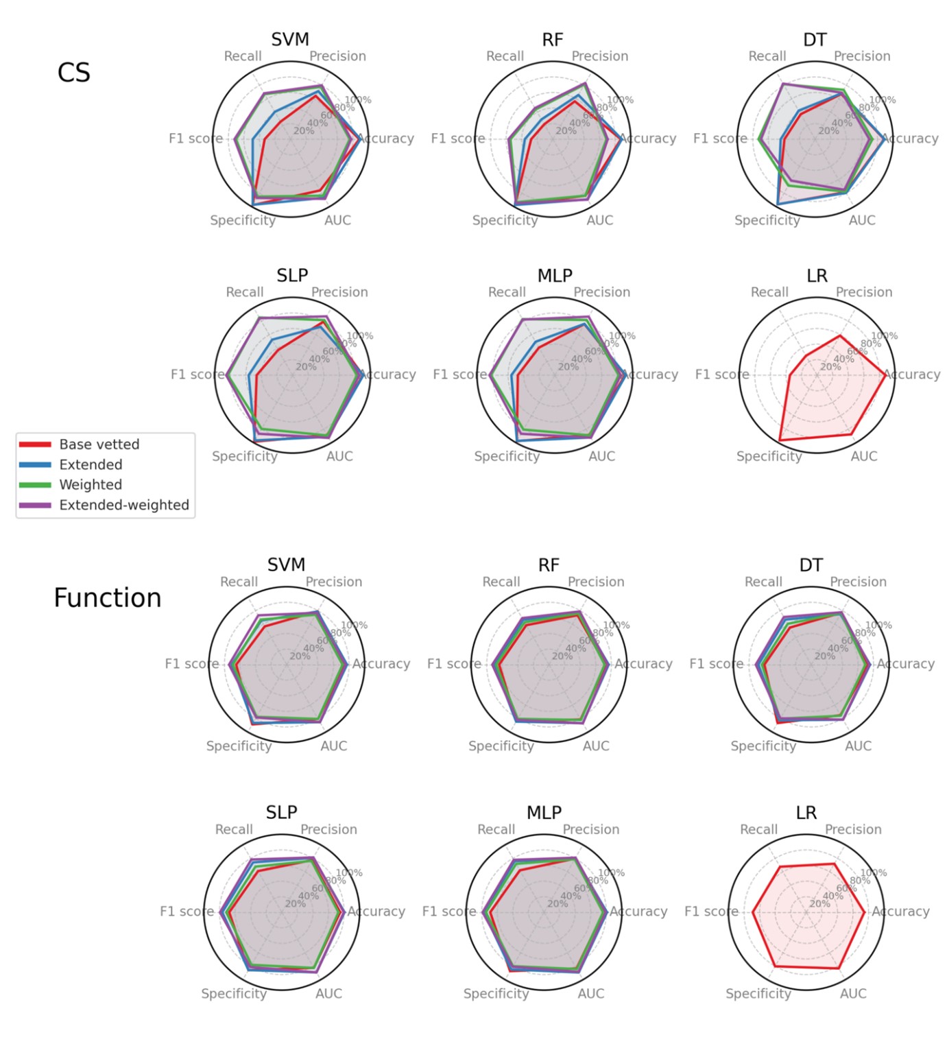
For CS classification, the median accuracy was 0.87 with IQR [0.78-0.89]. The highest accuracy means were seen in MLPε (0.91 ± 0.038), SLPε (0.91 ± 0.038), SLP (0.9 ± 0.034), MLP (0.9 ± 0.037), and the lowest mean in DTεw (0.7 ± 0.201) and RFw (0.69 ± 0.13). The median F1-scores was 0.56 with IQR [0.44-0.72]. The weighted and the extended-weighted models performed better, with the highest means seen in SLPεw (0.85 ± 0.095), MLPεw (0.84 ± 0.109), and the lowest mean seen in RF (0.28 ± 0.23). The median specificity was 0.97 with IQR [0.87-0.97]. Weight extension was associated with gains or no significant losses in specificity or AUC (Figures 2 & 3).
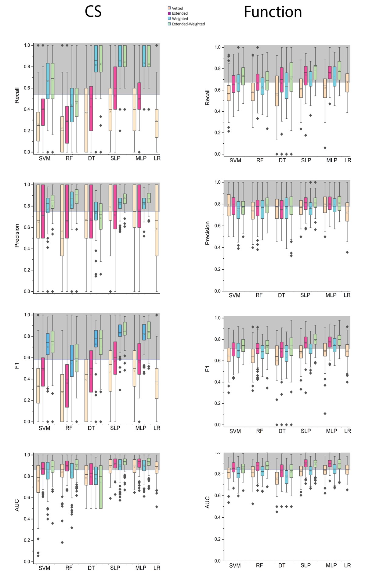
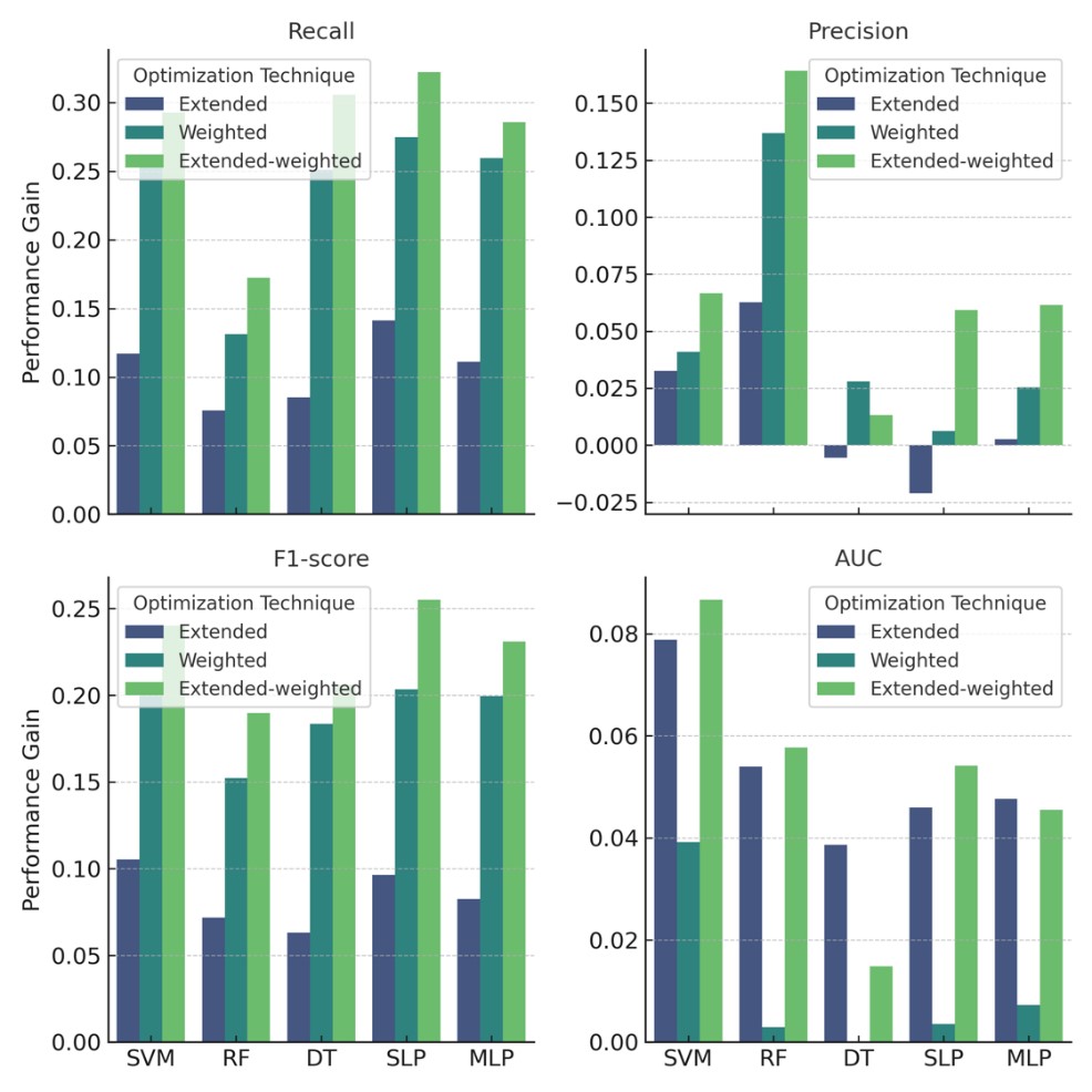
Figure 2 is Comparisons of the performance metrics between ML algorithms in classifying CS and function following weight adjustment and extension. Notice that the remarkable recall gains with weight extension did not correlate with losses in AUC. The grey area marks the space above the grand mean.
3.1.2. Function
The accuracy median of the model classifying function was 0.75 with IQR [0.73-0.77]. The highest accuracy means were seen in MLPε (0.81 ± 0.064), SLPε (0.81 ± 0.063), and the lowest in DTw (0.7 ± 0.119). The F1-score median was 0.7 with IQR [0.68-0.74]. The highest F1-scores were observed in SLPεw (0.79 ± 0.068), MLPεw (0.79 ± 0.072) and the lowest F1-scores in DT (0.6 ± 0.216). The optimized models had higher F1-scores than the basic ones, with the mean differences reaching 39.15% between RFεw and RF. The models were compared with a median specificity of 0.82 with IQR [0.8-0.86] (Figure 2). The highest specificity was seen in SVM (0.89 ± 0.077), and the lowest in SVMw (0.77 ± 0.102).
3.2. Connected Letter Charts
Commonly across both CS and function classifications, MLPε performed the best in accuracy (0.91 in CS, 0.81 in function). SLPεw was the best in precision (0.87 in CS, 0.81 in function) and F1-scores (0.85 in CS, 0.79 in function). For recall, SLPεw and MLPεw achieved the highest means (0.85 in CS, 0.78 in function, and 0.83 in CS, 0.78 in function, respectively). SLPεw, and MLPεw demonstrated the best performance in AUC 0.93 and 0.89, respectively. Regarding specificity, SVM outperformed others (0.98 in CS and 0.89 in function) (Table 1).
TABLE 1: Connected
letter chart results of multiple statistical comparisons between ML algorithms,
bolded blue represent the highest mean (value in parenthesis) and the grey
lowest mean (value in parenthesis), when more than
1 mean is present.
|
Top
connected letter chart |
Bottom
connected letter chart |
|||||
|
Central Sulcus |
Function |
Common |
Central Sulcus |
Function |
Common |
|
|
Accuracy |
MLPe (0.91), SLPe, SLP, MLP |
MLPe (0.81) |
MLPe (0.86) |
RFew, DTew, RFw (0.69) |
DTw
(0.7) |
- |
|
Precision |
SLPew
(0.87), MLPew |
SLPew
(0.81) |
SLPew
(0.84) |
RF (0.56) |
LR (0.72) |
- |
|
Recall |
SLPw
(0.86), SLPew, MLPw, DTew, MLPew, DTw |
SLPew (0.78), MLPew |
SLPew (0.82), MLPew |
RF
(0.22) |
DT
(0.55) |
- |
|
F1-score |
SLPew
(0.85),
MLPew,
SLPw |
SLPew
(0.79) |
SLPew
(0.82) |
RF (0.28) |
DT (0.6) |
- |
|
AUC |
SLPew (0.93), MLPew, MLPe |
MLPe (0.89), SLPew, SLPe, MLPew |
SLPew (0.91), MLPew (0.91), MLPe (0.91) |
DTew (0.75) |
DTw,
DT (0.75) |
- |
|
Specificity |
SLP (0.98),
SVM, MLP, RFe,
MLPe,
SVMe,
RF, SLPe,
DT, LR, DTe,
Rfew,
RFw |
SVM (0.89) |
SVM (0.94) |
DTew
(0.61) |
SVMw (0.77) |
- |
3.3. Weight-Extension Effect
Weight-extension notably enhanced precision, recall, and F1-score by 27.15%, 48.27%, and 39.15%, respectively, for CS or function classification. This resulted in an average 3.9% AUC gain for both. A positive correlation (r=0.71) was observed in performance gains between optimized and basic models for CS and function (Figure 3 & Supplementary Figure 4).
3.4. Comparison with LR
The comparison of each model with LR showed that the neural networks, particularly the optimized ones, had better performance than LR. The mean differences in recall between SLPεw and LR were 33.3% on average and a maximum of 55.8%. (Tables 2 & 3).
TABLE 2: Comparison
between models and LR presented as the average of mean differences between
central Sulcus and function. Blue-shaded values are statistically significant
gains, and grey-shaded values are statistically significant losses.
|
Accuracy |
Precision |
Recall |
F1 |
Specificity |
AUC |
||
|
SVM |
SVM |
ns |
ns |
ns |
ns |
ns |
ns |
|
SVMe |
ns |
ns |
ns |
ns |
ns |
ns |
|
|
SVMw |
ns |
ns |
ns |
ns |
ns |
ns |
|
|
SVMew |
ns |
ns |
ns |
ns |
ns |
ns |
|
|
RF |
RF |
ns |
ns |
ns |
ns |
ns |
ns |
|
RFe |
ns |
ns |
ns |
1.2% |
ns |
ns |
|
|
RFw |
ns |
ns |
ns |
ns |
ns |
ns |
|
|
RFew |
ns |
ns |
ns |
ns |
ns |
ns |
|
|
DT |
DT |
ns |
ns |
ns |
ns |
ns |
-8.7% |
|
DTe |
ns |
ns |
ns |
ns |
ns |
ns |
|
|
DTw |
-9.7% |
ns |
ns |
ns |
ns |
-8.7% |
|
|
DTew |
ns |
ns |
ns |
ns |
ns |
ns |
|
|
SLP |
SLP |
ns |
ns |
ns |
ns |
ns |
ns |
|
SLPe |
4.5% |
11.1% |
15.3% |
14.7% |
ns |
4.8% |
|
|
SLPw |
ns |
13.8% |
ns |
ns |
ns |
ns |
|
|
SLPew |
ns |
19.1% |
33.3% |
30.4% |
ns |
5.5% |
|
|
MLP |
MLP |
ns |
12.6% |
ns |
ns |
ns |
ns |
|
MLPe |
4.8% |
13% |
14.5% |
14.7% |
ns |
5.3% |
|
|
MLPw |
ns |
15.1% |
ns |
26.4% |
ns |
ns |
|
|
MLPew |
ns |
18.7% |
32% |
29.5% |
ns |
5.1% |
|
Ns:
non-significant.
TABLE 3: Comparison
between models and LR presented mean differences (maximum values) between
central Sulcus or function. Blue-shaded values are statistically significant
gains, and grey-shaded values are statistically significant losses.
Ns: non-significant.
3.5. Hyperparameter Testing
i) The original and hyper-tuned SVM models showed similar accuracy across all metrics (11 p-values between 0.07-0.82) except for AUC, where the original's AUC was notably higher (0.85 vs. 0.82, p <0.001).
ii) For RF, increasing the tree count from 100 to 1000 didn't significantly reduce misclassification regardless of input variables, with a consistent gains ratio median of 1 (IQR 1-1). However, a rise from 1 to 100 trees did improve rates, evidenced by a median gains ratio of 1.25 and an IQR of [1.26-1.64]. This implies that while boosting the number of trees enhances classifications initially, the impact diminishes after a certain point, underscoring the importance of computational efficiency.
iii) A positive correlation (r = 0.72) existed between added features and AUC up to 9 variables. After this, the correlation dwindled, stabilizing at 0.5, suggesting an optimal threshold for feature addition in the Random Forest model. This suggests that screening for feature co-linearity may aid efficiency [7].
iv) Comparing the conventional square root to 0.75 of total features per RF split, there was no significant accuracy difference for CS classification in metrics like accuracy, AUC, and precision (p-values 0.59-0.77). However, employing 0.75 features significantly improved recall (0.36 vs. 0.2, p<0.001). No significant metric differences were found for function (p range 0.33-0.7).
v) Comparing 2-layer models with 4 vs. 2 neurons each, no significant differences were observed in CS and function over 12 metrics (p range 0.03-0.97). This mirrors the stable performance seen with a 3-neuron SLP for binary classification.
4. Discussion
This study assessed various ML algorithms on two binary classifications using icEEG compared to standard functional mapping. We aimed to find the best ML algorithm by optimizing features and parameters. Results indicated that optimized neural networks excel in these classifications, with feature augmentation and data weighting boosting performance. Recall improvements reached 62% and 55.8% against LR. Using 10-fold cross-validation, we identified top models based on low misclassification rates. However, more than showcasing the best models can be misleading. Hence, we performed further analyses to discern single-electrode model differences. Our research highlights the strength of machine learning, specially optimized multi-layer perceptron, in quickly mapping the central sulcus and related sensorimotor functions via short sleep intracranial EEG data. This method is on par with traditional, time-consuming electrical simulation mapping techniques. Our findings emphasize machine learning's potential to advance patient care through efficient methods that reduce reliance on experts.
Some conceptual challenges exist; some relate to training machine learning against an average physician's performance, which is more art than science. We found value in employing outcome-validated training on a broad range of features often overlooked by classical statistical regression design leading to devising novel markers. A striking aspect was dealing with disease as outliers and rare occurrences-representative of unbalanced data sets. The accuracy paradox-a mismatch between accuracy goals set for machine-learning models versus their practical application-can hinder its implementation [16]. However, our paradox-aware optimization yielded significant gains up to 0.59 in recall when weighing for unbalanced data and extending the number of studied features. This compares favorably and practically to previous computational efforts reporting 78-83% sensitivities and 60-67% specificity, and much less AUCs [17, 18]. This also compares favorably to expert-driven multi-feature computational designs [7]. Unlike traditional ROC curves where effective point adjustment correlates with losses in specificity, our adjustment correlated with additional gains under the curve, along with recall and precision compared to base models. Awareness of this paradox and ways to optimize models is crucial while considering realistic applications of these techniques.
A strong positive correlation exists between the performance differences of vetted and extended weighted models in CS and function classification. This suggests that the effect of weight extension was consistent for both tasks, implying its benefits are broadly applicable across different classification tasks. Traditional diagnostic standards need reassessment. Exploring AI-driven computational biomarkers offers promise. Machines have the potential to surpass average physician judgments, a shift we should embrace. The robustness of our analyses emphasizes the importance of leveraging these insights for clinical challenges. With AI, we can enhance diagnosis and treatment for various medical issues.
5. Conclusion
Our study showcases the effectiveness of machine learning, specially optimized multilayer perceptron, in analyzing brief intracranial EEG data during sleep for multi-hour clinical procedures. This emphasizes AI's potential for binary decision-making and optimization's importance in addressing unbalanced data. Addressing this imbalance is crucial to prevent misinterpretation and navigate the accuracy paradox, facilitating AI's adoption in healthcare. Our findings advocate for deeper AI integration into healthcare and comparison with outcome-validated metrics, potentially harmonizing human evaluations with emerging technologies.
Author Contributions
Iktimal Alwan: Analysis of data and Manuscript preparation. Dennis D. Spencer: data collection, revision for intellectual content, and study supervision. Rafeed Alkawadri: Conceptualization of the study, data collection, data analysis, manuscript revision, and study supervision. The first author assumes responsibility for data integrity and analysis - access to data. All authors review the manuscript and approve the content.
Conflicts of Interest
None.
REFERENCES
[1] Matthew M Zack, Rosemarie Kobau
“National and State Estimates of the Numbers of Adults and Children with Active
Epilepsy - United States, 2015.” MMWR Morb Mortal Wkly Rep, vol. 66, no.
31, pp. 821-825, 2017. View at: Publisher Site | PubMed
[2] Zhibin Chen, Martin J Brodie, Danny
Liew, et al. “Treatment Outcomes in Patients With Newly Diagnosed Epilepsy
Treated With Established and New Antiepileptic Drugs: A 30-Year Longitudinal
Cohort Study.” JAMA Neurol, vol. 75, no. 3, pp. 279-286, 2018. View at: Publisher Site | PubMed
[3] Rafeed Alkawadri “Brain-Computer
Interface (BCI) Applications in Mapping of Epileptic Brain Networks Based on
Intracranial-EEG: An Update.” Front Neurosci, vol. 13, pp. 191, 2019.
View at: Publisher
Site | PubMed
[4] Nykan Mirchi, Nebras M Warsi,
Frederick Zhang, et al. “Decoding Intracranial EEG With Machine Learning: A
Systematic Review.” Front Hum Neurosci, vol. 16, pp. 913777, 2022. View
at: Publisher Site | PubMed
[5] Jiawei Han, Micheline Kamber, Jian
Pei “Data mining concepts and techniques third edition.” University of Illinois
at Urbana-Champaign Micheline Kamber Jian Pei Simon Fraser University, 2012.
[6] Iqbal H Sarker “Machine Learning:
Algorithms, Real-World Applications and Research Directions.” SN Comput Sci,
vol. 2, no. 3, pp. 160, 2021. View at: Publisher Site | PubMed
[7] Rafeed Alkawadri, Hitten P Zaveri,
Kevin N Sheth, et al. “Passive localization of the central sulcus during sleep
based on intracranial EEG.” Cereb Cortex, vol. 32, no. 17, pp.
3726-3735, 2022. View at: Publisher
Site | PubMed
[8] Trevor Hastie , Robert Tibshirani ,
Jerome Friedman “The elements of statistical learning: data mining, inference,
and prediction.” Springer Series in Statistics, vol. 2, 2009.
[9] Vladimir Vapnik “Estimation of
dependences based on empirical data.” Information Science and Statistics,
2006.
[10] Barry de Ville “Decision trees.” WIREs
Computational Statistics, vol. 5, no. 6, pp. 448-455, 2013. View at: Publisher Site
[11] Gérard Biau, Erwan Scornet “A random
forest guided tour.” Test, vol. 25, pp. 197-227, 2016. View at: Publisher Site
[12] Hebb, D. O “Hebb, D. O. Organization
of behavior. New York: Wiley, 1949, pp. 335” J Clin Psychol, vol. 6, no.
3, pp. 307, 1950. View at: Publisher
Site
[13] W S McCulloch, W Pitts “A logical
calculus of the ideas immanent in nervous activity. 1943.” Bull Math Biol,
vol. 5, no. 1-2, pp. 99-115, 1990. View at: PubMed
[14] Köhler Wolfgang “Gestalt psychology
today.” American psychologist, vol. 14, no. 12, pp. 727, 1959. View at: Publisher Site
[15] J. S. Cramer “The Origins of Logistic
Regression.” Tinbergen Institute Discussion Papers, 2002.
[16] Valverde-Albacete, F. J. &
Peláez-Moreno, C. “100% classification accuracy considered harmful: The
normalized information transfer factor explains the accuracy paradox.” PLoS
One, vol. 9, no. 1, pp. e84217, 2014. View at: Publisher Site | PubMed
[17] Jonathan D Breshears 1, Charles M Gaona, Jarod L Roland, et al. “Mapping sensorimotor cortex using slow cortical potential resting-state networks while awake and under anesthesia.” Neurosurgery, vol. 71, no. 2, pp. 305-316, 2012. View at: Publisher Site | PubMed
[18] Vernon L Towle, Leila Khorasani, Stephen Uftring, et al. “Noninvasive identification of human central sulcus: a comparison of gyral morphology, functional MRI, dipole localization, and direct cortical mapping.” Neuroimage, vol. 19, no. 3, pp. 684-697, 2003. View at: Publisher Site | PubMed